Calculating inertia tensors of shapes

Computing the inertia tensor of an arbitrary volume in 3D involves a complicated integral. For polytopes, the integral becomes especially complicated because the shape must be broken up into simplices in order to perform the calculation, and making the calculation numerically robust requires careful consideration of how best to perform the calculation. coxeter uses the best available algorithms for different shapes to minimize these errors, making it equally easy to compute moments of inertia for simple shapes like circles and complex ones like polyhedra.

import numpy as np
import rowan
from matplotlib import pyplot as plt
from mpl_toolkits import mplot3d

import coxeter

def plot_polyhedron(poly, include_tensor=False, length_scale=3):
    """Plot a polyhedron a provided set of matplotlib axes.

    The include_tensor parameter controls whether or not the axes
    of the inertia tensor are plotted. If they are, then the
    length_scale controls how much the axis vectors are extended,
    which is purely for visualization purposes.
    """
    fig, ax = plt.subplots(figsize=(6, 6), subplot_kw={"projection": "3d"})

    # Generate a triangulation for plot_trisurf.
    vertex_to_index = {tuple(v): i for i, v in enumerate(poly.vertices)}
    triangles = [
        [vertex_to_index[tuple(v)] for v in triangle]
        for triangle in poly._surface_triangulation()
    ]

    # Plot the triangulation to get faces, but without any outlines because outlining
    # the triangulation will include lines along faces where coplanar simplices intersect.
    verts = poly.vertices
    ax.plot_trisurf(
        verts[:, 0],
        verts[:, 1],
        verts[:, 2],
        triangles=triangles,
        # Make the triangles partly transparent.
        color=tuple([*plt.get_cmap("tab10").colors[4], 0.3]),
    )

    # Add lines manually.
    for face in poly.faces:
        verts = poly.vertices[face]
        verts = np.concatenate((verts, verts[[0]]))
        ax.plot(verts[:, 0], verts[:, 1], verts[:, 2], c="k", lw=0.4)

    # If requested, plot the axes of the inertia tensor.
    if include_tensor:
        centers = np.repeat(poly.center[np.newaxis, :], axis=0, repeats=3)
        arrows = poly.inertia_tensor * length_scale
        ax.quiver3D(
            centers[:, 0],
            centers[:, 1],
            centers[:, 2],
            arrows[:, 0],
            arrows[:, 1],
            arrows[:, 2],
            color="k",
            lw=3,
        )

    ax.view_init(elev=30, azim=-90)
    limits = np.array([ax.get_xlim3d(), ax.get_ylim3d(), ax.get_zlim3d()])
    center = np.mean(limits, axis=1)
    radius = 0.5 * np.max(limits[:, 1] - limits[:, 0])
    ax.set_xlim([center[0] - radius, center[0] + radius])
    ax.set_ylim([center[1] - radius, center[1] + radius])
    ax.set_zlim([center[2] - radius, center[2] + radius])
    ax.tick_params(which="both", axis="both", labelsize=0)
    fig.subplots_adjust(top=1, bottom=0, right=1, left=0, hspace=0, wspace=0)
    fig.tight_layout()

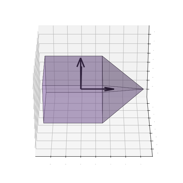
In this notebook, we will demonstrate the inertia tensor calculation using a square pyramid, a shape whose 3D orientation is easy to visualize. First, let’s see what this shape looks like.

vertices = np.array(
    [
        [0.0, 0.0, 1.073],
        [0.0, -0.707, -0.634],
        [0.0, -0.707, 0.366],
        [0.0, 0.707, -0.634],
        [0.0, 0.707, 0.366],
        [-0.707, 0.0, -0.634],
        [-0.707, 0.0, 0.366],
        [0.707, 0.0, -0.634],
        [0.707, 0.0, 0.366],
    ]
)
pyramid = coxeter.shapes.ConvexPolyhedron(vertices)

plot_polyhedron(pyramid)
print(pyramid.inertia_tensor.round(3))

[[ 0.27  0.   -0.  ]
 [ 0.    0.27  0.  ]
 [-0.    0.    0.19]]

Now let’s see what the axes of the inertia tensor are as calculated using coxeter. To make them more prominent, we’ll scale them since we’re not doing any physical calculations where the magnitude is important here. Additionally, we’ll rotate the shape so that it’s principal frame is not aligned to the coordinate axes to make it easier to see the axes of the inertia tensor.

rotated_pyramid = coxeter.shapes.ConvexPolyhedron(
    rowan.rotate([-0.6052796, 0.49886219, -0.21305172, 0.58256509], vertices)
)

plot_polyhedron(rotated_pyramid, include_tensor=True, length_scale=3)
print(rotated_pyramid.inertia_tensor.round(3))

[[ 0.214 -0.024 -0.028]
 [-0.024  0.26  -0.012]
 [-0.028 -0.012  0.257]]

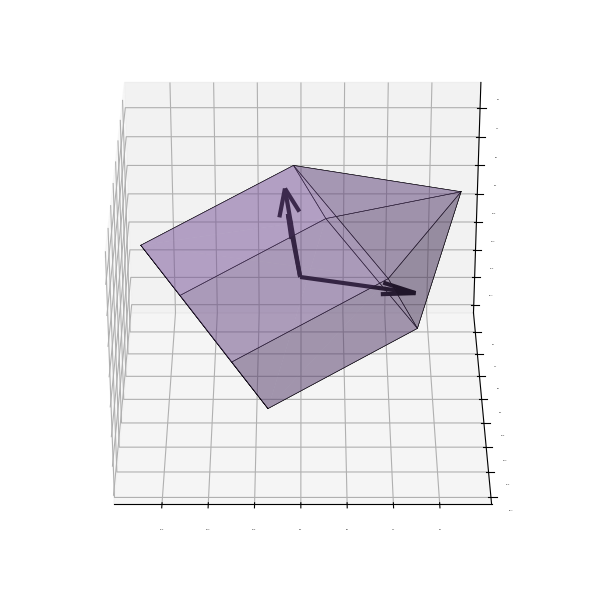
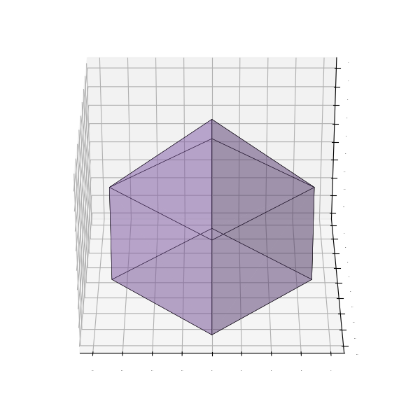
From this perspective, we can at least two of the axes quite well (the third vector pointing into the screen is largely obscured by the vector pointing up). It is often convenient to work with shapes in their principal frame, i.e. the frame in which the inertia tensor is diagonalized. coxeter makes it easy to diagonalize a shape with a single command.

rotated_pyramid.diagonalize_inertia()
plot_polyhedron(rotated_pyramid, include_tensor=True)
print(rotated_pyramid.inertia_tensor.round(3))

[[ 0.19 -0.   -0.  ]
 [-0.    0.27  0.  ]
 [-0.    0.    0.27]]